Google Docs

Nov 14, 2021·2 min read Programming

library(googlesheets4)
library(sf)
library(opencage) # for geocoding addresses
library(usethis)
library(hrbrthemes) # hrbrmstr/hrbrthemes
library(tidyverse)
library(kableExtra)
library(rnaturalearth)
library(tmap)
library(ggthemes)

# usethis::edit_r_environ() # add Opencage API to your .Renviron file

# Add a line OPENCAGE_KEY="xxxxxxxxxxxxxxxxxxxxxxxxxxxxxxx"
# Before you exit, make sure your .Renviron ends with a blank line, then save and close it.
# Restart RStudio after modifying .Renviron in order to load the API key into memory. 
# To check everything worked, go to console and type 
# Sys.getenv("OPENCAGE_KEY")


googlesheets4::gs4_auth() # google sheets authorisation

#load countries_visited googlesheets
countries_visited <- read_sheet("https://docs.google.com/spreadsheets/d/14k4xrwrMRfabnyqQ2y_mTNdf-gT5KBDMAAS42H44V7E/edit?usp=sharing
") 

geocoded <- countries_visited %>% 
  mutate(
    address_geo = purrr::map(country, opencage_forward, limit=1) # the beauty of purrr:map()
  ) %>% 
  unnest_wider(address_geo) %>% # opencage returns a list, hence we unnest it...
  unnest(results) %>% # look inside the results that opencage returns
  rename(lat = geometry.lat, # rename latitude/longitude to lat/lng
         lng = geometry.lng) %>% 
  select(country, lat, lng) # just select country, latitude, longitude

geocoded %>% 
  kable()%>%  # print a table with geocoded addresses
  kable_styling(bootstrap_options = c("striped", "hover", "condensed", "responsive"))

# we will use the rnatural earth package to get a medium resolution 
# vector map of world countries excl. Antarctica
world <- ne_countries(scale = "medium", returnclass = "sf") %>%
  filter(name != "Antarctica") 

st_geometry(world) # what is the geometry?

## Geometry set for 240 features 
## Geometry type: MULTIPOLYGON
## Dimension:     XY
## Bounding box:  xmin: -180 ymin: -58.49229 xmax: 180 ymax: 83.59961
## CRS:           +proj=longlat +datum=WGS84 +no_defs +ellps=WGS84 +towgs84=0,0,0
## First 5 geometries:

# CRS:            +proj=longlat +datum=WGS84 +no_defs +ellps=WGS84 +towgs84=0,0,0

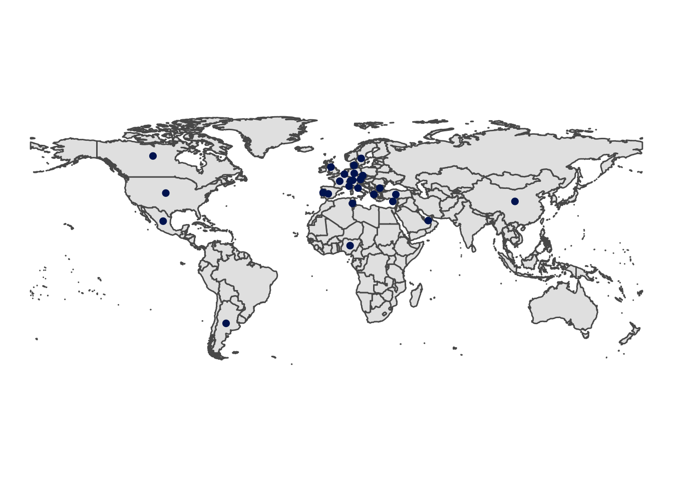
ggplot(data = world) +
  geom_sf() + # the first two lines just plot the world shapefile
  geom_point(data = geocoded, # then we add points
             aes(x = lng, y = lat), 
             size = 2, 
             colour = "#001e62") +
  theme_void()

world_visited <- left_join(world, geocoded,  by=c("admin" = "country" )) %>% 
    mutate(visited = if_else (!is.na(lat), "visited", "not visited")
  )

ggplot(world_visited)+
  geom_sf(aes(fill=visited),     
          show.legend = FALSE)+    # no legend
  scale_fill_manual(values=c('#f0f0f0', '#3182bd'))+
  coord_sf(datum = NA) +
  theme_void()+
  labs(title="Which countries have I travelled to?")+
  theme_ipsum_rc(grid="", strip_text_face = "bold") +
  NULL